Power of Function Composition, Non Linear Activation, XOR problem
At its most basic level, a neural network is a computational graph that performs compositions of simpler functions to provide a more complex function. Much of the power of deep learning arises from the fact that repeated composition of multiple nonlinear functions has significant expressive power. Even though the single composition of a large number of squashing functions can approximate almost any function, this approach will require an extremely large number of units (i.e., parameters) of the network. This increases the capacity of the network, which causes overfitting unless the data set is extremely large. Much of the power of deep learning arises from the fact that the repeated composition of certain types of functions increases the representation power of the network, and therefore reduces the parameter space required for learning.
Not all base functions are equally good at achieving this goal. In fact, the nonlinear squashing functions used in neural networks are not arbitrarily chosen, but are carefully designed because of certain types of properties. For example, imagine a situation in which the identity activation function is used in each layer, so that only linear functions are computed. In such a case, the resulting neural network is no stronger than a single-layer, linear network.A multi-layer network that uses only the identity activation function in all its layers reduces to a single-layer network performing linear regression.A similar result holds true for binary target variables. In the special case, where all layers use identity activation and the final layer uses a single output with sign activation for prediction, the multilayer neural network reduces to the perceptron.
This result shows that deep networks largely make sense only when the activation functions in intermediate layers are non-linear. Typically, the functions like sigmoid and tanh are squashing functions in which the output is bounded within an interval, and the gradients are largest near zero values. For large absolute values of their arguments, these functions are said to reach saturation where increasing the absolute value of the argument further does not change its value significantly. This type of function in which values do not vary significantly at large absolute values of their arguments is shared by another family of functions, referred to as Gaussian kernels, which are commonly used in non-parametric density estimation:
$\Phi(v)=exp(-v^2/2)$
The only difference is that Gaussian kernels saturate to 0 at large values of their argument, whereas functions like sigmoid and tanh can also saturate to values of +1 and −1. It is well known in the literature on density estimation that the sum of many small Gaussian kernels can be used to approximate any density function.Density functions have a special nonnegative structure in which extremes of the data distribution always saturate to zero density, and therefore the underlying kernels also show the same behavior.A similar principle holds true (more generally) for squashing functions in which the linear combination of many small activation functions can be used to approximate an arbitrary function; however, squashing functions do not saturate to zero in order to handle arbitrary behavior at extreme values. The universal approximation result of neural networks posits that a linear combination of sigmoid units (and/or most other reasonable squashing functions) in a single hidden layer can be used to approximate any function well. Note that the linear combination can be performed by a single output node. Therefore, a two-layer network is sufficient as long as the number of hidden units is large enough. However, some kind of basic non-linearity in the activation function is always required in order to model the turns and twists in an arbitrary function. To understand this point, note that all 1-dimensional functions can be approximated as a sum of scaled/translated step functions and most of the activation functions (e.g., sigmoid) look awfully like step functions.
This basic idea is the essence of the universal approximation theorem of neural networks. In fact, the proof of the ability of squashing functions to approximate any function is conceptually similar to that of kernels at least at an intuitive level. However, the number of base functions required to reach a high level of approximation can be extremely large in both cases, potentially increasing the data-centric requirements to an unmanageable level. For this reason, shallow networks face the persistent problem of overfitting. The universal approximation theorem asserts the ability to well-approximate the function implicit in the training data, but makes no guarantee about whether the function can be generalized to unseen test data.
The Importance of Nonlinear Activation
The previous section provides a concrete proof of the fact that a neural network with only linear activations does not gain from increasing the number of layers in it. For example, consider the two-class data set illustrated in Figure , which is represented in two dimensions denoted by $x_1$ and $x_2$. There are two instances, $A$ and $B$, of the class denoted by ‘*’ with coordinates (1, 1) and (−1, 1), respectively. There is also a single instance $B$ of the class denoted by ‘+’ with coordinates (0, 1), A neural network with only linear activations will never be able to classify the training data perfectly because the points are not linearly separable.

On the other hand, consider a situation in which the hidden units have ReLU activation, and they learn the two new features $h_1$ and $h_2$, which are as follows:
$h_1 = max\{x_1, 0\}$
$h_2 = max\{−x_1, 0\}$
Note that these goals can be achieved by using appropriate weights from the input to hidden layer, and also applying a ReLU activation unit. The latter achieves the goal of thresholding negative values to 0. We have indicated the corresponding weights in the neural network shown in Figure . We have shown a plot of the data in terms of $h_1$ and $h_2$ in the same figure. The coordinates of the three points in the 2-dimensional hidden layer are {(1, 0), (0, 1), (0, 0)}. It is immediately evident that the two classes become linearly separable in terms of the new hidden representation. In a sense, the task of the first layer was representation learning to enable the solution of the problem with a linear classifier.
Therefore, if we add a single linear output layer to the neural network, it will be able to classify these training instances perfectly. The key point is that the use of the nonlinear ReLU function is crucial in ensuring this linear separability. Activation functions enable nonlinear mappings of the data, so that the embedded points can become linearly separable.
In fact, if both the weights from hidden to output layer are set to 1 with a linear activation function, the output O will be defined as follows:
$O = h_1 + h_2$
This simple linear function separates the two classes because it always takes on the value of 1 for the two points labeled ‘*’ and takes on 0 for the point labeled ‘+’. Therefore, much of the power of neural networks is hidden in the use of activation functions. The weights shown in Figure will need to be learned in a data-driven manner, although there are many alternative choices of weights that can make the hidden representation linearly separable.Therefore, the learned weights may be different than the ones shown in Figure above, if actual training is performed. Nevertheless, in the case of the perceptron, there is no choice of weights at which one could hope to classify this training data set perfectly because the data set is not linearly separable in the original space. In other words, the activation functions enable nonlinear transformations of the data, that become increasingly powerful with multiple layers. A sequence of nonlinear activations imposes a specific type of structure on the learned model, whose power increases with the depth of the sequence (i.e., number of layers in the neural network).
XOR
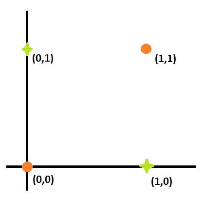
Another classical example is the XOR function in which the two points {(0, 0), (1, 1)} belong to one class, and the other two points {(1, 0), (0, 1)} belong to the other class.It is possible to use ReLU activation to separate these two classes as well, although bias neurons will be needed in this case .The XOR function was one of the motivating factors for designing multilayer networks and the ability to train them. The XOR function is considered a litmus test to determine the basic feasibility of a particular family of neural networks to properly predict nonlinearly separable classes. Although we have used the ReLU activation function above for simplicity, it is possible to use most of the other nonlinear activation functions to achieve the same goals.Here $sigmoid$ function is used.
This is a binary classification problem. Hence, supervised learning is a better way to solve it. In this case, we will be using perceptrons. Uni layered perceptrons can only work with linearly separable data. But in the following diagram drawn in accordance with the truth table of the XOR loical operator, we can see that the data is NOT linearly separable.


Comments
Post a Comment