Implementation of two layer neural network- XOR with sigmoid activation function

Implementing logic gates using neural networks help understand the mathematical computation by which a neural network processes its inputs to arrive at a certain output. This neural network will deal with the XOR logic problem. An XOR (exclusive OR gate) is a digital logic gate that gives a true output only when both its inputs differ from each other.

THE NEURAL NETWORK MODEL

As mentioned before, the neural network needs to produce two different decision planes to linearly separate the input data based on the output patterns. This is achieved by using the concept of hidden layers. The neural network will consist of one input layer with two nodes (X1,X2); one hidden layer with two nodes (since two decision planes are needed); and one output layer with one node (Y). Hence, the neural network looks like this: 

THE SIGMOID NEURON

To implement an XOR gate,  Sigmoid Neurons  nodes are used in the neural network. The characteristics of a Sigmoid Neuron are:

1. Can accept real values as input.

2. The value of the activation is equal to the weighted sum of its inputs
i.e. $\sum w_i x_i$

3. The output of the sigmoid neuron is a function of the sigmoid function, which is also known as a logistic regression function. The sigmoid function is a continuous function which outputs values between 0 and 1:

THE LEARNING ALGORITHM

The information of a neural network is stored in the interconnections between the neurons i.e. the weights. A neural network learns by updating its weights according to a learning algorithm that helps it converge to the expected output. The learning algorithm is a principled way of changing the weights and biases based on the loss function.

1.Initialize the weights and biases randomly.

2.Iterate over the data

    i. Compute the predicted output using the sigmoid function

    ii. Compute the loss using the square error loss function

    iii. $W(new) = W(old) — α ∆W$

    iv. $B(new) = B(old) — α ∆B$

3.Repeat until the error is minimal

This is a fairly simple learning algorithm consisting of only arithmetic operations to update the weights and biases. The algorithm can be divided into two parts: the forward pass and the backward pass also known as “backpropagation.”

The forward pass involves compute the predicted output, which is a function of the weighted sum of the inputs given to the neurons:

The predicted_output needs to be compared with the expected_output. Based on this comparison, the weights for both the hidden layers and the output layers are changed using backpropagation. Backpropagation is done using the Gradient Descent algorithm.

GRADIENT DESCENT

The loss function of the sigmoid neuron is the squared error loss. If we plot the loss/error against the weights we get something like this:

Our goal is to find the weight vector corresponding to the point where the error is minimum i.e. the minima of the error gradient. And here is where calculus comes into play.

THE MATH BEHIND GRADIENT DESCENT

Error can be simply written as the difference between the predicted outcome and the actual outcome. Mathematically:

where $t$ is the targeted/expected output and $y$ is the predicted output.However, is it fair to assign different error values for the same amount of error? For example, the absolute difference between -1 and 0 & 1 and 0 is the same, however the above formula would sway things negatively for the outcome that predicted -1. To solve this problem, we use square error loss.(Note modulus is not used, as it makes it harder to differentiate). Further, this error is divided by 2, to make it easier to differentiate, as we’ll see in the following steps.

Since, there may be many weights contributing to this error, we take the partial derivative, to find the minimum error, with respect to each weight at a time. The change in weights are different for the output layer weights (W31 & W32) and different for the hidden layer weights (W11, W12, W21, W22).

Let the outer layer weights be $w_o$ while the hidden layer weights be $w_h$.

We’ll first find $∆W$ for the outer layer weights. Since the outcome is a function of activation and further activation is a function of weights, by chain rule:

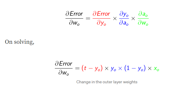
Note that for $X_o$ is nothing but the output from the hidden layer nodes. This output from the hidden layer node is again a function of the activation and correspondingly a function of weights. Hence, the chain rule expands for the hidden layer weights:

This process is repeated until the predicted_output converges to the expected_output. It is easier to repeat this process a certain number of times (iterations/epochs) rather than setting a threshold for how much convergence should be expected.

Python Implementation of XOR neural network

import numpy as np
# creating the input array
X=np.array([[0,0],[0,1],[1,0],[1,1]])
print ('\n Input:')
print(X)

# creating the output array
y=np.array([[0],[1],[1],[0]])
print ('\n Actual Output:')
print(y)


# defining the Sigmoid Function
def sigmoid (x):
    return 1/(1 + np.exp(-x))

# derivative of Sigmoid Function
def derivatives_sigmoid(x):
    return x * (1 - x)

# initializing the variables
epoch=50000 # number of training iterations
lr=0.1 # learning rate

inputlayer_neurons = X.shape[1] # number of features in data set
hiddenlayer_neurons = 2# number of hidden layers neurons
output_neurons = 1 # number of neurons at output layer

# initializing weight and bias

wh=np.random.uniform(size=(inputlayer_neurons,hiddenlayer_neurons))
bh=np.random.uniform(size=(1,hiddenlayer_neurons))
wout=np.random.uniform(size=(hiddenlayer_neurons,output_neurons))
bout=np.random.uniform(size=(1,output_neurons))

print("Initial weight and bias in hidden layer")
print(wh)
print(bh)

print("Initial weight and bias in output layer")
print(wout)
print(bout)

# training the model
for i in range(epoch):
    #Forward Propogation
    hidden_layer_input1=np.dot(X,wh)

    hidden_layer_input=hidden_layer_input1 + bh

    hiddenlayer_activations = sigmoid(hidden_layer_input)

    output_layer_input1=np.dot(hiddenlayer_activations,wout)

    output_layer_input= output_layer_input1+ bout

    output = sigmoid(output_layer_input)

#Backpropagation
    E = y-output
    slope_output_layer = derivatives_sigmoid(output)

    slope_hidden_layer = derivatives_sigmoid(hiddenlayer_activations)

    d_output = E * slope_output_layer

    Error_at_hidden_layer = d_output.dot(wout.T)

    d_hiddenlayer = Error_at_hidden_layer * slope_hidden_layer

    wout += hiddenlayer_activations.T.dot(d_output) *lr

    bout += np.sum(d_output, axis=0,keepdims=True) *lr

    wh += X.T.dot(d_hiddenlayer) *lr

    bh += np.sum(d_hiddenlayer, axis=0,keepdims=True) *lr


print("Final weight and bias in the hidden layer")
print(wh)
print(bh)

print("Final weight and bias in the output layer")
print(wout)
print(bout)

print ('\n Output from the model:')
print (output)

Output

Input:
[[0 0]
 [0 1]
 [1 0]
 [1 1]]

 Actual Output:
[[0]
 [1]
 [1]
 [0]]
Initial weight and bias in hiiden layer
[[0.56793119 0.71140962]
 [0.97757389 0.50994691]]
[[0.80262921 0.42020226]]
Initial weight and bias in output layer
[[0.79450035]
 [0.49973622]]
[[0.46820481]]
Final weight and bias in the hidden layer
[[6.49234202 4.59127701]
 [6.48302122 4.58903129]]
[[-2.88301491 -7.04372803]]
Final weight and bias in the output layer
[[  9.60527993]
 [-10.3063663 ]]
[[-4.4428787]]

 Output from the model:
[[0.01902526]
 [0.98356434]
 [0.98357436]
 [0.01702198]]